Lab 4 - QA/QC

GOAL AND BACKGROUND

The goal of this lab was to learn how to perform relative and absolute QA/QC, along with doing manual QA/QC on classification.


METHODS

LP360  and the LP360 extension in ArcMap was used for this data processing. First, point cloud density was checked by creating a map that showed low density areas. According to this, point density was acceptable throughout the study area.

Next, relative accuracy was assessed. A map was created that displayed differences in elevation. This was used for swath-to-swath analysis. For this analysis, seamlines were created along flat, unobstructed areas within the overlap lines.

Next, absolute accuracy was assessed. This was done for both vertical and horizontal accuracy. Checkpoint locations for each were imported from a spreadsheet. Vertical checkpoints were referenced for measured values vs. values from the LiDAR data. Horizontal checkpoints were displayed on the map and refenced with the LiDAR data.

Manual QA/QC of classification errors involved looking through the study area and flagging classification errors. Once this was done, these errors were rectified using manual classification tools such as classifying in the profile window.


RESULTS

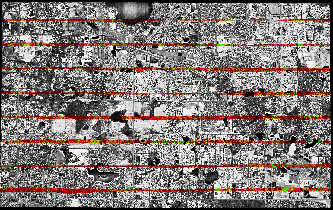
The map created in relative accuracy assessment showing differences in elevation is shown below. The horizontal lines are overlap of flight lines. The results from swath-to-swath analysis showed few areas above the maximum height value.

The results from the absolute accuracy showed the data was good. Vertical checkpoints were all within 0.10 cm error. Horizontal checkpoint analysis determined the data was in class 0 for both X and Y accuracy.

Manual QA/QC was done through much of the data, an example of this is shown below. The error was first flagged, as shown in the first image, then rectified, as shown in the second. The flag was removed after fixing the error.

SOURCES

Data obtained from Cyril Wilson for use in 358 LiDAR course.

Lab 3 - Vegetation Classification

GOAL AND BACKGROUND

The goal of this lab was to learn how to classify vegetation in LiDAR data. The vegetation would be classified by low, medium, and high vegetation. High noise would also be classified in this process. QA/QC will be necessary to minimize error.


METHODS

LP360 was used for this data processing. A height filter was used to classify data into either low, medium, or high vegetation. If the points were above the high vegetation threshold, they would be classified as high noise. Only unclassified points were chosen, since vegetation is the last to be classified.


RESULTS

The study area after classification is shown below. The newly classified vegetation is shown as green.

Below are a few examples of closer views of classification within the study area. First is a building that was shown in the previous posts, now with classified vegetation.

Below is a view of some residential housing in the study area. The algorithms had some trouble differentiating between houses and vegetation at some points, especially when it involved overlap. Manual cleanup was used after the algorithm.

SOURCES

Data obtained from Cyril Wilson for use in 358 LiDAR course.

Lab 2 - Building Classification

GOAL AND BACKGROUND

The goal of this lab was to learn how to classify buildings in LiDAR data. This would be done with the data that ground was already classified, which was done in the first lab. Some basic QA/QC would be necessary to minimize error.

METHODS

LP360 was used for this lab. A planar point filter was used to classify buildings. Basic parameters were set, such as a height filter. The purpose of the height filter was to cut out planar surfaces low enough that would not be buildings, such as cars, and high enough that high noise would be ignored. Other parameters, such as minimum edge plane, grow window area, and N fit were also set and adjusted to best filter the data.

The results are shown and discussed below.

RESULTS

The entire study area after building classification is shown below. Buildings are classified by red, ground by orange, water by blue, and gray areas are unclassified, which at this point is vegetation.

Below are a few examples of closer views of buildings within the study area. First is a building that was shown as previously unclassified in the lab 1 post, now classified accurately.

The next image shows residential housing that was classified. Note that residential housing had trouble being classified with the algorithm, so a lot of manual cleanup was necessary.

SOURCES

Data obtained from Cyril Wilson for use in 358 LiDAR course.